Training the Jetbot: Ground Truth#
With the environment defined, we can now start modifying our observations and rewards in order to train a policy to act as a controller for the Jetbot. As a user, we would like to be able to specify the desired direction for the Jetbot to drive, and have the wheels turn such that the robot drives in that specified direction as fast as possible. How do we achieve this with Reinforcement Learning (RL)? If you want to cut to the end and checkout the result of this stage of the walk through, checkout this branch of the tutorial repository!
Expanding the Environment#
The very first thing we need to do is create the logic for setting commands for each Jetbot on the stage. Each command will be a unit vector, and
we need one for every clone of the robot on the stage, which means a tensor of shape [num_envs, 3]. Even though the Jetbot only navigates in the
2D plane, by working with 3D vectors we get to make use of all the math utilities provided by Isaac Lab.
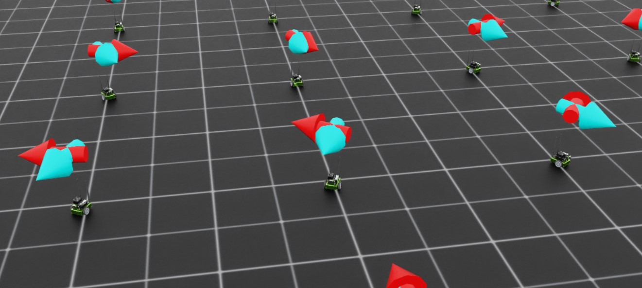
It would also be a good idea to setup visualizations, so we can more easily tell what the policy is doing during training and inference.
In this case, we will define two arrow VisualizationMarkers: one to represent the “forward” direction of the robot, and one to
represent the command direction. When the policy is fully trained, these arrows should be aligned! Having these visualizations in place
early helps us avoid “silent bugs”: issues in the code that do not cause it to crash.
To begin, we need to define the marker config and then instantiate the markers with that config. Add the following to the global scope of isaac_lab_tutorial_env.py
from isaaclab.markers import VisualizationMarkers, VisualizationMarkersCfg
from isaaclab.utils.assets import ISAAC_NUCLEUS_DIR
import isaaclab.utils.math as math_utils

def define_markers() -> VisualizationMarkers:
    """Define markers with various different shapes."""
    marker_cfg = VisualizationMarkersCfg(
        prim_path="/Visuals/myMarkers",
        markers={
                "forward": sim_utils.UsdFileCfg(
                    usd_path=f"{ISAAC_NUCLEUS_DIR}/Props/UIElements/arrow_x.usd",
                    scale=(0.25, 0.25, 0.5),
                    visual_material=sim_utils.PreviewSurfaceCfg(diffuse_color=(0.0, 1.0, 1.0)),
                ),
                "command": sim_utils.UsdFileCfg(
                    usd_path=f"{ISAAC_NUCLEUS_DIR}/Props/UIElements/arrow_x.usd",
                    scale=(0.25, 0.25, 0.5),
                    visual_material=sim_utils.PreviewSurfaceCfg(diffuse_color=(1.0, 0.0, 0.0)),
                ),
        },
    )
    return VisualizationMarkers(cfg=marker_cfg)
The VisualizationMarkersCfg defines USD prims to serve as the “marker”. Any prim will do, but generally you want to keep markers as simple as possible because the cloning of markers occurs at runtime on every time step.
This is because the purpose of these markers is for debug visualization only and not to be a part of the simulation: the user has full control over how many markers to draw when and where.
NVIDIA provides several simple meshes on our public nucleus server, located at ISAAC_NUCLEUS_DIR, and for obvious reasons we choose to use arrow_x.usd.
For a more detailed example of using VisualizationMarkers checkout the markers.py demo!
Code for the markers.py demo
  1# Copyright (c) 2022-2026, The Isaac Lab Project Developers (https://github.com/isaac-sim/IsaacLab/blob/main/CONTRIBUTORS.md).
  2# All rights reserved.
  3#
  4# SPDX-License-Identifier: BSD-3-Clause
  5
  6"""This script demonstrates different types of markers.
  7
  8.. code-block:: bash
  9
 10    # Usage
 11    ./isaaclab.sh -p scripts/demos/markers.py
 12
 13"""
 14
 15"""Launch Isaac Sim Simulator first."""
 16
 17import argparse
 18
 19from isaaclab.app import AppLauncher
 20
 21# add argparse arguments
 22parser = argparse.ArgumentParser(description="This script demonstrates different types of markers.")
 23# append AppLauncher cli args
 24AppLauncher.add_app_launcher_args(parser)
 25# parse the arguments
 26args_cli = parser.parse_args()
 27
 28# launch omniverse app
 29app_launcher = AppLauncher(args_cli)
 30simulation_app = app_launcher.app
 31
 32"""Rest everything follows."""
 33
 34import torch
 35
 36import isaaclab.sim as sim_utils
 37from isaaclab.markers import VisualizationMarkers, VisualizationMarkersCfg
 38from isaaclab.sim import SimulationContext
 39from isaaclab.utils.assets import ISAAC_NUCLEUS_DIR, ISAACLAB_NUCLEUS_DIR
 40from isaaclab.utils.math import quat_from_angle_axis
 41
 42
 43def define_markers() -> VisualizationMarkers:
 44    """Define markers with various different shapes."""
 45    marker_cfg = VisualizationMarkersCfg(
 46        prim_path="/Visuals/myMarkers",
 47        markers={
 48            "frame": sim_utils.UsdFileCfg(
 49                usd_path=f"{ISAAC_NUCLEUS_DIR}/Props/UIElements/frame_prim.usd",
 50                scale=(0.5, 0.5, 0.5),
 51            ),
 52            "arrow_x": sim_utils.UsdFileCfg(
 53                usd_path=f"{ISAAC_NUCLEUS_DIR}/Props/UIElements/arrow_x.usd",
 54                scale=(1.0, 0.5, 0.5),
 55                visual_material=sim_utils.PreviewSurfaceCfg(diffuse_color=(0.0, 1.0, 1.0)),
 56            ),
 57            "cube": sim_utils.CuboidCfg(
 58                size=(1.0, 1.0, 1.0),
 59                visual_material=sim_utils.PreviewSurfaceCfg(diffuse_color=(1.0, 0.0, 0.0)),
 60            ),
 61            "sphere": sim_utils.SphereCfg(
 62                radius=0.5,
 63                visual_material=sim_utils.PreviewSurfaceCfg(diffuse_color=(0.0, 1.0, 0.0)),
 64            ),
 65            "cylinder": sim_utils.CylinderCfg(
 66                radius=0.5,
 67                height=1.0,
 68                visual_material=sim_utils.PreviewSurfaceCfg(diffuse_color=(0.0, 0.0, 1.0)),
 69            ),
 70            "cone": sim_utils.ConeCfg(
 71                radius=0.5,
 72                height=1.0,
 73                visual_material=sim_utils.PreviewSurfaceCfg(diffuse_color=(1.0, 1.0, 0.0)),
 74            ),
 75            "mesh": sim_utils.UsdFileCfg(
 76                usd_path=f"{ISAAC_NUCLEUS_DIR}/Props/Blocks/DexCube/dex_cube_instanceable.usd",
 77                scale=(10.0, 10.0, 10.0),
 78            ),
 79            "mesh_recolored": sim_utils.UsdFileCfg(
 80                usd_path=f"{ISAAC_NUCLEUS_DIR}/Props/Blocks/DexCube/dex_cube_instanceable.usd",
 81                scale=(10.0, 10.0, 10.0),
 82                visual_material=sim_utils.PreviewSurfaceCfg(diffuse_color=(1.0, 0.25, 0.0)),
 83            ),
 84            "robot_mesh": sim_utils.UsdFileCfg(
 85                usd_path=f"{ISAACLAB_NUCLEUS_DIR}/Robots/ANYbotics/ANYmal-C/anymal_c.usd",
 86                scale=(2.0, 2.0, 2.0),
 87                visual_material=sim_utils.GlassMdlCfg(glass_color=(0.0, 0.1, 0.0)),
 88            ),
 89        },
 90    )
 91    return VisualizationMarkers(marker_cfg)
 92
 93
 94def main():
 95    """Main function."""
 96    # Load kit helper
 97    sim_cfg = sim_utils.SimulationCfg(dt=0.01, device=args_cli.device)
 98    sim = SimulationContext(sim_cfg)
 99    # Set main camera
100    sim.set_camera_view([0.0, 18.0, 12.0], [0.0, 3.0, 0.0])
101
102    # Spawn things into stage
103    # Lights
104    cfg = sim_utils.DomeLightCfg(intensity=3000.0, color=(0.75, 0.75, 0.75))
105    cfg.func("/World/Light", cfg)
106
107    # create markers
108    my_visualizer = define_markers()
109
110    # define a grid of positions where the markers should be placed
111    num_markers_per_type = 5
112    grid_spacing = 2.0
113    # Calculate the half-width and half-height
114    half_width = (num_markers_per_type - 1) / 2.0
115    half_height = (my_visualizer.num_prototypes - 1) / 2.0
116    # Create the x and y ranges centered around the origin
117    x_range = torch.arange(-half_width * grid_spacing, (half_width + 1) * grid_spacing, grid_spacing)
118    y_range = torch.arange(-half_height * grid_spacing, (half_height + 1) * grid_spacing, grid_spacing)
119    # Create the grid
120    x_grid, y_grid = torch.meshgrid(x_range, y_range, indexing="ij")
121    x_grid = x_grid.reshape(-1)
122    y_grid = y_grid.reshape(-1)
123    z_grid = torch.zeros_like(x_grid)
124    # marker locations
125    marker_locations = torch.stack([x_grid, y_grid, z_grid], dim=1)
126    marker_indices = torch.arange(my_visualizer.num_prototypes).repeat(num_markers_per_type)
127
128    # Play the simulator
129    sim.reset()
130    # Now we are ready!
131    print("[INFO]: Setup complete...")
132
133    # Yaw angle
134    yaw = torch.zeros_like(marker_locations[:, 0])
135    # Simulate physics
136    while simulation_app.is_running():
137        # rotate the markers around the z-axis for visualization
138        marker_orientations = quat_from_angle_axis(yaw, torch.tensor([0.0, 0.0, 1.0]))
139        # visualize
140        my_visualizer.visualize(marker_locations, marker_orientations, marker_indices=marker_indices)
141        # roll corresponding indices to show how marker prototype can be changed
142        if yaw[0].item() % (0.5 * torch.pi) < 0.01:
143            marker_indices = torch.roll(marker_indices, 1)
144        # perform step
145        sim.step()
146        # increment yaw
147        yaw += 0.01
148
149
150if __name__ == "__main__":
151    # run the main function
152    main()
153    # close sim app
154    simulation_app.close()
Next, we need to expand the initialization and setup steps to construct the data we need for tracking the commands as well as the marker positions and rotations. Replace the contents of
_setup_scene with the following
def _setup_scene(self):
    self.robot = Articulation(self.cfg.robot_cfg)
    # add ground plane
    spawn_ground_plane(prim_path="/World/ground", cfg=GroundPlaneCfg())
    # clone and replicate
    self.scene.clone_environments(copy_from_source=False)
    # add articulation to scene
    self.scene.articulations["robot"] = self.robot
    # add lights
    light_cfg = sim_utils.DomeLightCfg(intensity=2000.0, color=(0.75, 0.75, 0.75))
    light_cfg.func("/World/Light", light_cfg)

    self.visualization_markers = define_markers()

    # setting aside useful variables for later
    self.up_dir = torch.tensor([0.0, 0.0, 1.0]).cuda()
    self.yaws = torch.zeros((self.cfg.scene.num_envs, 1)).cuda()
    self.commands = torch.randn((self.cfg.scene.num_envs, 3)).cuda()
    self.commands[:,-1] = 0.0
    self.commands = self.commands/torch.linalg.norm(self.commands, dim=1, keepdim=True)

    # offsets to account for atan range and keep things on [-pi, pi]
    ratio = self.commands[:,1]/(self.commands[:,0]+1E-8)
    gzero = torch.where(self.commands > 0, True, False)
    lzero = torch.where(self.commands < 0, True, False)
    plus = lzero[:,0]*gzero[:,1]
    minus = lzero[:,0]*lzero[:,1]
    offsets = torch.pi*plus - torch.pi*minus
    self.yaws = torch.atan(ratio).reshape(-1,1) + offsets.reshape(-1,1)

    self.marker_locations = torch.zeros((self.cfg.scene.num_envs, 3)).cuda()
    self.marker_offset = torch.zeros((self.cfg.scene.num_envs, 3)).cuda()
    self.marker_offset[:,-1] = 0.5
    self.forward_marker_orientations = torch.zeros((self.cfg.scene.num_envs, 4)).cuda()
    self.command_marker_orientations = torch.zeros((self.cfg.scene.num_envs, 4)).cuda()
Most of this is setting up the book keeping for the commands and markers, but the command initialization and the yaw calculations are worth diving into. The commands
are sampled from a multivariate normal distribution via torch.randn with the z component fixed to zero and then normalized to unit length. In order to point our
command markers along these vectors, we need to rotate the base arrow mesh appropriately. This means we need to define a quaternion that will rotate the arrow
prim about the z axis by some angle defined by the command. By convention, rotations about the z axis are called a “yaw” rotation (akin to roll and pitch).
Luckily for us, Isaac Lab provides a utility to generate a quaternion from an axis of rotation and an angle: isaaclab.utils.math.quat_from_axis_angle(), so the only
tricky part now is determining that angle.

The yaw is defined about the z axis, with a yaw of 0 aligning with the x axis and positive angles opening counterclockwise. The x and y components of the command vector define the tangent of this angle, and so we need the arctangent of that ratio to get the yaw.
Now, consider two commands: Command A is in quadrant 2 at (-x, y), while command B is in quadrant 4 at (x, -y). The ratio of the
y component to the x component is identical for both A and B. If we do not account for this, then some of our command arrows will be
pointing in the opposite direction of the command! Essentially, our commands are defined on [-pi, pi] but arctangent is
only defined on [-pi/2, pi/2].
To remedy this, we add or subtract pi from the yaw depending on the quadrant of the command.
ratio = self.commands[:,1]/(self.commands[:,0]+1E-8) #in case the x component is zero
gzero = torch.where(self.commands > 0, True, False)
lzero = torch.where(self.commands < 0, True, False)
plus = lzero[:,0]*gzero[:,1]
minus = lzero[:,0]*lzero[:,1]
offsets = torch.pi*plus - torch.pi*minus
self.yaws = torch.atan(ratio).reshape(-1,1) + offsets.reshape(-1,1)
Boolean expressions involving tensors can have ambiguous definitions and pytorch will throw errors regarding this. Pytorch provides
various methods to make the definitions explicit. The method torch.where produces a tensor with the same shape as the input
with each element of the output is determined by the evaluation of that expression on only that element. A reliable way to handle
boolean operations with tensors is to simply produce boolean indexing tensors and then represent the operation algebraically, with AND
as multiplication and OR as addition, which is what we do above. This is equivalent to the pseudocode:
yaws = torch.atan(ratio)
yaws[commands[:,0] < 0 and commands[:,1] > 0] += torch.pi
yaws[commands[:,0] < 0 and commands[:,1] < 0] -= torch.pi
Next we have the method for actually visualizing the markers. Remember, these markers aren’t scene entities! We need to “draw” them whenever we want to see them.
def _visualize_markers(self):
    # get marker locations and orientations
    self.marker_locations = self.robot.data.root_pos_w
    self.forward_marker_orientations = self.robot.data.root_quat_w
    self.command_marker_orientations = math_utils.quat_from_angle_axis(self.yaws, self.up_dir).squeeze()

    # offset markers so they are above the jetbot
    loc = self.marker_locations + self.marker_offset
    loc = torch.vstack((loc, loc))
    rots = torch.vstack((self.forward_marker_orientations, self.command_marker_orientations))

    # render the markers
    all_envs = torch.arange(self.cfg.scene.num_envs)
    indices = torch.hstack((torch.zeros_like(all_envs), torch.ones_like(all_envs)))
    self.visualization_markers.visualize(loc, rots, marker_indices=indices)
The visualize method of VisualizationMarkers is like this “draw” function. It accepts tensors for the spatial
transformations of the markers, and a marker_indices tensor to specify which marker prototype to use for each marker. So
long as the first dimension of all of these tensors match, this function will draw those markers with the specified transformations.
This is why we stack the locations, rotations, and indices.
Now we just need to call _visualize_markers on the pre physics step to make the arrows visible. Replace _pre_physics_step with the following
def _pre_physics_step(self, actions: torch.Tensor) -> None:
  self.actions = actions.clone()
  self._visualize_markers()
The last major modification before we dig into the RL training is to update the _reset_idx method to account for the commands and markers. Whenever we reset an environment,
we need to generate a new command and reset the markers. The logic for this is already covered above. Replace the contents of _reset_idx with the following:
def _reset_idx(self, env_ids: Sequence[int] | None):
    if env_ids is None:
        env_ids = self.robot._ALL_INDICES
    super()._reset_idx(env_ids)

    # pick new commands for reset envs
    self.commands[env_ids] = torch.randn((len(env_ids), 3)).cuda()
    self.commands[env_ids,-1] = 0.0
    self.commands[env_ids] = self.commands[env_ids]/torch.linalg.norm(self.commands[env_ids], dim=1, keepdim=True)

    # recalculate the orientations for the command markers with the new commands
    ratio = self.commands[env_ids][:,1]/(self.commands[env_ids][:,0]+1E-8)
    gzero = torch.where(self.commands[env_ids] > 0, True, False)
    lzero = torch.where(self.commands[env_ids]< 0, True, False)
    plus = lzero[:,0]*gzero[:,1]
    minus = lzero[:,0]*lzero[:,1]
    offsets = torch.pi*plus - torch.pi*minus
    self.yaws[env_ids] = torch.atan(ratio).reshape(-1,1) + offsets.reshape(-1,1)

    # set the root state for the reset envs
    default_root_state = self.robot.data.default_root_state[env_ids]
    default_root_state[:, :3] += self.scene.env_origins[env_ids]

    self.robot.write_root_state_to_sim(default_root_state, env_ids)
    self._visualize_markers()
And that’s it! We now generate commands and can visualize it the heading of the Jetbot. We are ready to start tinkering with the observations and rewards.